One of the ways to represent the results of an experiment with one user-controlled variable (independent variable) and another variable that supposedly changes with the changes in the independent variable (the dependent variable), is the scatter-plot. If the data-points are uncorrelated they will be dispersed equally across four corners of the plot and if they are correlated they will be along the diagonal. It is called positive correlation when they are along the rising diagonal and negative correlation when they are on the falling diagonal.
However, this data is of the co-ordinate form (x,y) and therefore two dimensional. Now suppose that we are looking at more than one dependent variable. Then it could be that our data will become 3 dimensional with the co-ordinates of (x,y,z). Now 3-D data can still be observed by plotting (x,y) & (x,z) but if there are more dimensions like 4,7 or 12 you can see that it will become hard to plot and observe. In that case we will be looking for a scatterplot that shows the variation in the data but it will be harder to find.
Enter Principal Components Analysis, PCA needs you to format/formalize your data as a matrix where the columns represent the various dependent variables. Each column represents a dimension in space, so each of your rows is a point in N dimensional space where N is the number of columns/variables in the matrix.
So the first step to doing a PCA is to center your data using the mean. Then you calculate the covariance matrix of this mean centered data and then find the eigen-values and the corresponding eigenvectors and sort the eigenvectors by the magnitude of their eigen-values. These eigenvectors represent the projection of the data-points into a lower dimensional space that preserves the maximum amount of variation in the data. The magnitude of the eigenvalues with respect to the total represents the proportion of variance explained by rotating the data by the corresponding eigenvector.
So, yeah, that is the explanation every text on PCA gives you, so what am I telling differently here?
A couple of things, first, mean centering the data would bring the data to the origin of the co-ordinate system with the mean being the origin instead of the data-points being arbitrarily located at one corner of the graph. So, geometrically, when mean-centered, all of your observations are defined in values which when squared and added and then square-rooted would represent their Euclidean distance from the origin.
Next, what does it mean to calculate the co-variance matrix?.
Co-variance is a measure of how two or more set of data-points/random variables vary with each other. If you go through the post on Correlation: Nuts, Bolts and an Exploded view, you will understand how co-variance measures, (in an un-normalized fashion), how much two random variables co-vary.
Variance is also called the second moment, so co-variance would be the second moment for two sets of data-points and would measure how fast the two data-points vary with respect to each other. Doesn't that sound like something that is familiar from calculus? the rate of change of a variable is expressed as the derivative isn't it? So is the co-variance matrix some sort of a matrix of derivatives?. Turns out that moments of data are analogous to the concept of derivatives of functions.

To make matters more fun, we come to the problem of computing eigenvalues and eigenvectors. The eigenvectors of a certain matrix are vectors that when multiplied with the matrix are not changed (i.e their co-ordinates do not change, they don't get rotated or translated) only their length changes. Length of a vector, assuming that we have mean-centered everything before this computation step, is simply the Euclidean distance from the origin (0,0,0...) which would be the square-root of the sum of squares of the co-ordinates. So length is a scalar quantity and the eigenvector is simply scaled by another scalar when you multiply the matrix with the eigenvector. In this case that particular scalar is the eigenvalues. So every eigenvector has its corresponding eigenvalue which indicates, how much the length of that vector would change when multiplied by the matrix.

So we calculate something called the characteristic polynomial for the covariance matrix with the yet-to-be-computed eigenvalues subtracted from the diagonal entries. The characteristic polynomial is basically the determinant of this matrix.

After we have the characteristic polynomial, we equate it to zero and calculate the eigenvalues. For those of you familiar with calculus, finding the first derivative and equating to zero and solving for the values is familiar as the computation of the maxima of a function. In this case, our function is the characteristic polynomial and the eigenvalues are simply the roots of that polynomial which maximize that function. Since the co-variance matrix is positive definite, there exists only a single, unique, minimum (if you flip the function by multiplying everything by -1, it becomes a maximum) and the eigen-values are defined at those points.
So what is the determinant here? according to geometrical intuition, determinants are areas (in higher dimensions, volumes) of the space spanned by the vectors of the matrix for which the determinant is being calculated. So, here, the determinant of the characteristic polynomial gives us a measure of the volume spanned by the vectors of the co-variance matrix and the eigenvalues give us the values by which each vector is shifted along each axes to maximize the volume spanned by the set of vectors.


So the eigenvectors which correspond to these eigenvalues are co-ordinates along which the proportion of scaling described by the corresponding eigenvalue is observed for the data.
So when you rotate the data such that they lie along these eigenvectors, they will describe the maximum about of variance in them. Essentially, the data points are rotated to a new set of co-ordinates where the maximum amount of variation present in the data is represented.
For intuitiveness, let's imagine that our data is an ellipsoid/egg, not a circle/sphere, so that it has two directions which have different variations/spreads. Later we will generalize it to a scalene ellipsoid which looks more like a bar of soap and has different spreads across different axes.
So ideally, if PCA is able to find the directions with the maximum variance then, for an ellipse it should find the major and minor semi-axes.
Now for some practical programming exercises.
Various texts on PCA will tell you that doing a PCA on your data rotates the data-points in such a way that you are able to visualize the maximum amount of variance in your data. So for now to make this intuitive, let us put together a data-set of 3 dimensions (because 2-dimensions can be visualized using a scatterplot). So we will be making a 3-D ellipse, often called an ellipsoid of data-points such that we can see it using an interactive 3-D plot that is available in R under the package rgl (installation instructions in the post on Brownian motion).
So we start with formulating a function for an ellipsoid. A 3-D ellipsoid would have co-ordinates (x,y,z) and the axes would be (a,b,c). The equation would be.
in R we type
ellipsoid<-function(xyz,abc,radius){
ellipse<-(xyz[,1]^2/abc[1]^2)+(xyz[,2]^2/abc[2]^2)+(xyz[,3]^2/abc[3]^2)
ellipsis<-which(ellipse<=radius)
return(xyz[ellipsis,])
}
So R newbies, this function uses a few shortcuts now. I'm passing the data as a matrix and indexing it in the body of the function to extract the respective (x,y,z) co-ordinates and sending the semi-axes as a vector of numbers. Compared to earlier posts this will be a little more of brevity. However the meaning stays the same and you will see it soon enough.
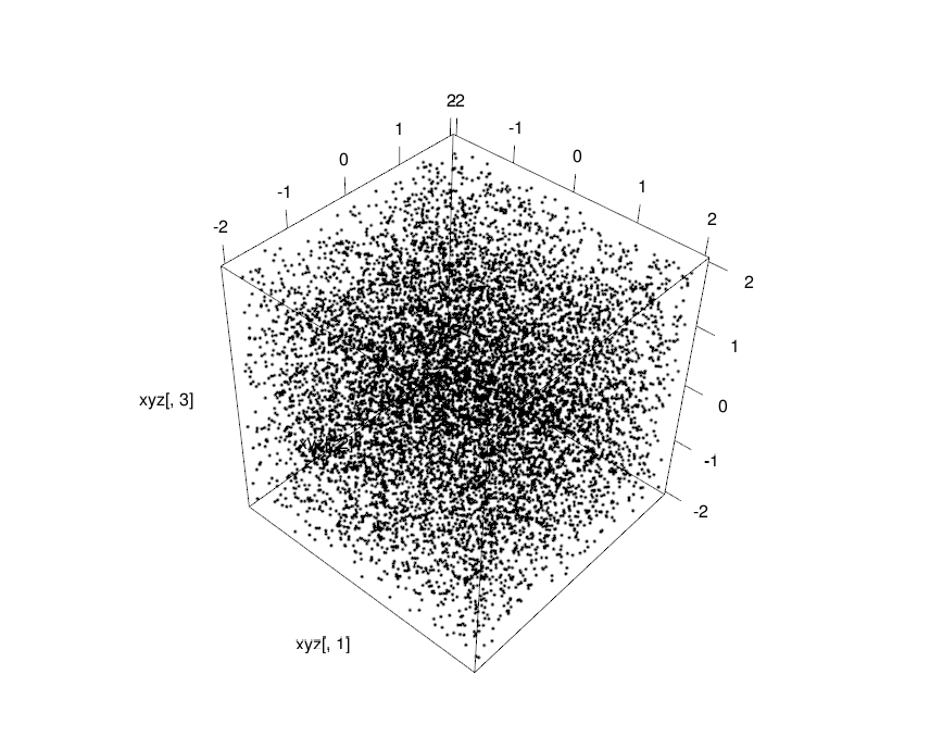
So here is what are going to do, we start with a box peppered with points every where uniformly, that will be our random cloud of data.
library(rgl)
xyz<-matrix(runif(30000,-2,2),10000,3)
plot3d(xyz[,1],xyz[,2],xyz[,3])
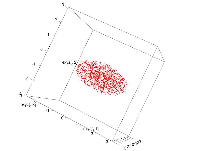
Then we transform it into an ellipsoid of points using the function ellipsoid which we just wrote. This ellipsoid will be our high-dimensional data. Although it is not really high-dimensional and you can very well use scatterplots to see what is happening but for the sake of argument, let us say that it is high-dimensional and we are unable to view it.
exyz<-ellipsoid(xyz,abc=c(2,1,1),radius=1)
plot3d(exyz[,1],exyz[,2],exyz[,3],xlim=c(-3,3),ylim=c(-3,3),zlim=c(-3,3),col="red")
 Now with this ellipsoidal cloud of points we will perform a principal
components analysis. Since PCA gives us vectors called Principal
Components which describe the greatest amount of variance in the data,
for an ellipse the PC's would be the semi-axes. There after we will see that
tweaking the length of the semi-axes (the values of a,b & c) will
show their reflection in the amount of variance in the principal
components.
Now with this ellipsoidal cloud of points we will perform a principal
components analysis. Since PCA gives us vectors called Principal
Components which describe the greatest amount of variance in the data,
for an ellipse the PC's would be the semi-axes. There after we will see that
tweaking the length of the semi-axes (the values of a,b & c) will
show their reflection in the amount of variance in the principal
components.
So first I'll just briefly talk about ellipsoids, ellipsoids can have different shapes depending on the length of the semi-axes (a,b,c). As a special case, if all three semi-axes are of the same length (1,1,1) then the ellipsoid actually becomes a sphere.If one of them is about twice as long as the other two which are equal (2,1,1) then the ellipsoid becomes egg-shaped and is called a prolate spheroid, similarly it could become an egg which is wider than it is tall and that would be an oblate spheroid which is what the Earth is like, being squashed at the Poles. A rare case is when a>b>c, there is a convention of ordering in the semi-axes, so a is the semi-axes along x, b is along y and c is along z. That rare case looks like a computer mouse and is called a tri-axial or scalene ellipse.

Code for scalene ellipsoid:
plot3d(ellipsoid(xyz,abc=c(1,2,3),radius=0.5),xlim=c(-3,3),ylim=c(-3,3),zlim=c(-3,3),col="red")
Why am I talking about ellipses here? because data with multiple dependent variables forms an ellipsoid in higher dimensions. Or at least the limiting case of normally distributed data would be an ellipse (oblate,prolate,spherical or scalene), because uniformly scattered points would have to be uniformly distributed if they are to be seen as evenly spread throughout the co-ordinates, which your data wouldn't be unless it was just random noise.
So knowing from theory that PCA rotates the data in such a way that we can see maximum variation, for an ellipsoid, the directions for maximum variation would be along the semi-axes right?
We needed to know the different kinds of ellipses and the above information will help us track how the variance described by the Principal Components change when we modify the length of the axes. So here we also need a convenient function to be able to tweak the parameters quickly and view them as well. Let us, for a short time, be really horrible programmers and make a function that displays the shape of the ellipsoid or does a principal components analysis with the relevant plots depending on what we feel we need to see.
Ellipsoid3D_PCA<-function(xyz,abc,radius,mode=NULL){
require(rgl)
pointcloud<-ellipsoid(xyz,abc,radius)
if(mode=="pcaPCplot"){
trypca<-princomp(pointcloud)
print(trypca)
biplot(trypca,cex=0.4)
}
if(mode=="3dPlot"){
plot3d(pointcloud[,1],pointcloud[,2],pointcloud[,3],xlim=c(-3,3),ylim=c(-3,3),zlim=c(-3,3))
}
if(length(mode)==0)
{
print("Mode is missing : use 3dPlot or pcaPCplot")
}
}
Now this function simplifies a lot of typing and helps you to quickly modify parameters by repeating the commands using the UP Arrow key.
Ellipsoid3D_PCA(xyz,abc=c(2,1,1),1,mode="pcaPCplot")
So PCA doesn't really care what length you chose for the semi-axes, it will always find the longest semi-axes as the first PC and the second longest as the second PC and the third longest semi-axes as the third PC. PCA will give you the same result even if you re-ordered the axes sizes like this.
Ellipsoid3D_PCA(xyz,abc=c(1,1,2),1,mode="pcaPCplot")
So the semi axes are like an averaging line which runs through the cloud of points and spans the maximum amount of points of the ellipsoid as possible along each of the independent co-ordinates x,y and z. By independent I mean that the x,y and z co-ordinates cannot be expressed in terms of each other. There is no linear relationship that would allow you to express one axis in terms of one or more of the others. This is a concept called orthogonality.
Principal Components are orthogonal to each other and are made up of linear combinations of the variables in the matrix (the columns). So, a principal component tells you how much of the variance that you see in your data can be described in terms of orthogonal axes that are composed of linear combinations of the variables in your experiment. So, in terms of biology, if one of your experiments is very noisy and has data scattered throughout the co-ordinates, it would contribute considerably to the principal components.
Now PCA is also said to be a method for dimensionality reduction. So you can reduce the number of dimensions in your data while retaining the maximum amount of variation that defines your data. So how would that work, what does dimensionality reduction mean?
Dimensionality here would be the number of variables in your experiment. So generally experiments are represented in the form of a numeric matrix where the rows represent the entities being experimented and observed and the columns represent the different perturbations that have been applied. Here is where the question that you are asking becomes important. So is your question, "what are the experiments which describe the maximum amount of variance in my data?" or is it, "what are the entities which describe the maximum amount of variance in my data?".
If it is the first, then your dimensions are "experiments", else you have to take the transpose of your matrix such that "experiments" comes on the rows and "entities" come on the columns.
So how can you reduce dimensionality, you may ask, because obviously, the number of experiments that we have done is fixed, you may say "I'm not going to remove the results of one experiment that I did just so that my data becomes manageable. I want all my experiments to be factored in!".
What if I told you that maybe, a bunch of experiments that you did, despite all the hard work that went into them, do not contribute anything in terms of new results. Not philosophically! but actually they do not give any new numbers that might be statistically analyzed to get interesting results because they all say the same thing numerically speaking, they are collinear and therefore one of them describes the variation just as well as the other of the bunch do.
"Well, I'm still not throwing them out!", you say and rightly so, we don't need to throw them out, we can still make another column/experiment that combines the bunch of these columns into one column that contains all the data in the bunch but expressed as a linear weighted sum of the individual experiments of the bunch.
This weighting of the experiments allows you to retain all the experiments and their results but you end up re-weighting them in terms of the amount of information that they contribute to your data. Information here is defined as variance, so coming from where we considered variance to be noise in experiments, we now consider variance to be a sign that something is happening in our data which we can't directly quantify in a numerical, pair-wise comparison but we can see that it changes the amount of variation observed in the data. So the variance observed is considered to be a result of the perturbation.
So, the eigen-vectors that you get after the PCA decomposition are a mapping of your original data matrix into a sub-space with lower amount of dimensions where the number of dimensions have been reduced by taking dimensions which are linear combinations of the original dimensions. So you have managed to express most of the significant variation in your data in the form of a matrix which is much smaller than what you started out with. This is what it means when it is said that PCA is used for dimensionality reduction.
We'll see a more hands-on approach to PCA in the next installment to this post. Mull over everything you've seen and learned here and try to check out other resources on PCA to see if you've gained a better understanding of what is going on, Also try out functions other than ellipsoids and see how PCA behaves for them. Increase the number of dimensions so that you now only have a 3-D projection of say a 7-D data-set. Play with parameters, axes values and have fun.
However, this data is of the co-ordinate form (x,y) and therefore two dimensional. Now suppose that we are looking at more than one dependent variable. Then it could be that our data will become 3 dimensional with the co-ordinates of (x,y,z). Now 3-D data can still be observed by plotting (x,y) & (x,z) but if there are more dimensions like 4,7 or 12 you can see that it will become hard to plot and observe. In that case we will be looking for a scatterplot that shows the variation in the data but it will be harder to find.
Enter Principal Components Analysis, PCA needs you to format/formalize your data as a matrix where the columns represent the various dependent variables. Each column represents a dimension in space, so each of your rows is a point in N dimensional space where N is the number of columns/variables in the matrix.
So the first step to doing a PCA is to center your data using the mean. Then you calculate the covariance matrix of this mean centered data and then find the eigen-values and the corresponding eigenvectors and sort the eigenvectors by the magnitude of their eigen-values. These eigenvectors represent the projection of the data-points into a lower dimensional space that preserves the maximum amount of variation in the data. The magnitude of the eigenvalues with respect to the total represents the proportion of variance explained by rotating the data by the corresponding eigenvector.
So, yeah, that is the explanation every text on PCA gives you, so what am I telling differently here?
A couple of things, first, mean centering the data would bring the data to the origin of the co-ordinate system with the mean being the origin instead of the data-points being arbitrarily located at one corner of the graph. So, geometrically, when mean-centered, all of your observations are defined in values which when squared and added and then square-rooted would represent their Euclidean distance from the origin.
Next, what does it mean to calculate the co-variance matrix?.
Co-variance is a measure of how two or more set of data-points/random variables vary with each other. If you go through the post on Correlation: Nuts, Bolts and an Exploded view, you will understand how co-variance measures, (in an un-normalized fashion), how much two random variables co-vary.
Variance is also called the second moment, so co-variance would be the second moment for two sets of data-points and would measure how fast the two data-points vary with respect to each other. Doesn't that sound like something that is familiar from calculus? the rate of change of a variable is expressed as the derivative isn't it? So is the co-variance matrix some sort of a matrix of derivatives?. Turns out that moments of data are analogous to the concept of derivatives of functions.
To make matters more fun, we come to the problem of computing eigenvalues and eigenvectors. The eigenvectors of a certain matrix are vectors that when multiplied with the matrix are not changed (i.e their co-ordinates do not change, they don't get rotated or translated) only their length changes. Length of a vector, assuming that we have mean-centered everything before this computation step, is simply the Euclidean distance from the origin (0,0,0...) which would be the square-root of the sum of squares of the co-ordinates. So length is a scalar quantity and the eigenvector is simply scaled by another scalar when you multiply the matrix with the eigenvector. In this case that particular scalar is the eigenvalues. So every eigenvector has its corresponding eigenvalue which indicates, how much the length of that vector would change when multiplied by the matrix.
So we calculate something called the characteristic polynomial for the covariance matrix with the yet-to-be-computed eigenvalues subtracted from the diagonal entries. The characteristic polynomial is basically the determinant of this matrix.
After we have the characteristic polynomial, we equate it to zero and calculate the eigenvalues. For those of you familiar with calculus, finding the first derivative and equating to zero and solving for the values is familiar as the computation of the maxima of a function. In this case, our function is the characteristic polynomial and the eigenvalues are simply the roots of that polynomial which maximize that function. Since the co-variance matrix is positive definite, there exists only a single, unique, minimum (if you flip the function by multiplying everything by -1, it becomes a maximum) and the eigen-values are defined at those points.
So what is the determinant here? according to geometrical intuition, determinants are areas (in higher dimensions, volumes) of the space spanned by the vectors of the matrix for which the determinant is being calculated. So, here, the determinant of the characteristic polynomial gives us a measure of the volume spanned by the vectors of the co-variance matrix and the eigenvalues give us the values by which each vector is shifted along each axes to maximize the volume spanned by the set of vectors.
So the eigenvectors which correspond to these eigenvalues are co-ordinates along which the proportion of scaling described by the corresponding eigenvalue is observed for the data.
So when you rotate the data such that they lie along these eigenvectors, they will describe the maximum about of variance in them. Essentially, the data points are rotated to a new set of co-ordinates where the maximum amount of variation present in the data is represented.
For intuitiveness, let's imagine that our data is an ellipsoid/egg, not a circle/sphere, so that it has two directions which have different variations/spreads. Later we will generalize it to a scalene ellipsoid which looks more like a bar of soap and has different spreads across different axes.
So ideally, if PCA is able to find the directions with the maximum variance then, for an ellipse it should find the major and minor semi-axes.
Now for some practical programming exercises.
Various texts on PCA will tell you that doing a PCA on your data rotates the data-points in such a way that you are able to visualize the maximum amount of variance in your data. So for now to make this intuitive, let us put together a data-set of 3 dimensions (because 2-dimensions can be visualized using a scatterplot). So we will be making a 3-D ellipse, often called an ellipsoid of data-points such that we can see it using an interactive 3-D plot that is available in R under the package rgl (installation instructions in the post on Brownian motion).
So we start with formulating a function for an ellipsoid. A 3-D ellipsoid would have co-ordinates (x,y,z) and the axes would be (a,b,c). The equation would be.
in R we type
ellipsoid<-function(xyz,abc,radius){
ellipse<-(xyz[,1]^2/abc[1]^2)+(xyz[,2]^2/abc[2]^2)+(xyz[,3]^2/abc[3]^2)
ellipsis<-which(ellipse<=radius)
return(xyz[ellipsis,])
}
So R newbies, this function uses a few shortcuts now. I'm passing the data as a matrix and indexing it in the body of the function to extract the respective (x,y,z) co-ordinates and sending the semi-axes as a vector of numbers. Compared to earlier posts this will be a little more of brevity. However the meaning stays the same and you will see it soon enough.
So here is what are going to do, we start with a box peppered with points every where uniformly, that will be our random cloud of data.
library(rgl)
xyz<-matrix(runif(30000,-2,2),10000,3)
plot3d(xyz[,1],xyz[,2],xyz[,3])
Then we transform it into an ellipsoid of points using the function ellipsoid which we just wrote. This ellipsoid will be our high-dimensional data. Although it is not really high-dimensional and you can very well use scatterplots to see what is happening but for the sake of argument, let us say that it is high-dimensional and we are unable to view it.
exyz<-ellipsoid(xyz,abc=c(2,1,1),radius=1)
plot3d(exyz[,1],exyz[,2],exyz[,3],xlim=c(-3,3),ylim=c(-3,3),zlim=c(-3,3),col="red")
So first I'll just briefly talk about ellipsoids, ellipsoids can have different shapes depending on the length of the semi-axes (a,b,c). As a special case, if all three semi-axes are of the same length (1,1,1) then the ellipsoid actually becomes a sphere.If one of them is about twice as long as the other two which are equal (2,1,1) then the ellipsoid becomes egg-shaped and is called a prolate spheroid, similarly it could become an egg which is wider than it is tall and that would be an oblate spheroid which is what the Earth is like, being squashed at the Poles. A rare case is when a>b>c, there is a convention of ordering in the semi-axes, so a is the semi-axes along x, b is along y and c is along z. That rare case looks like a computer mouse and is called a tri-axial or scalene ellipse.
Code for scalene ellipsoid:
plot3d(ellipsoid(xyz,abc=c(1,2,3),radius=0.5),xlim=c(-3,3),ylim=c(-3,3),zlim=c(-3,3),col="red")
Why am I talking about ellipses here? because data with multiple dependent variables forms an ellipsoid in higher dimensions. Or at least the limiting case of normally distributed data would be an ellipse (oblate,prolate,spherical or scalene), because uniformly scattered points would have to be uniformly distributed if they are to be seen as evenly spread throughout the co-ordinates, which your data wouldn't be unless it was just random noise.
So knowing from theory that PCA rotates the data in such a way that we can see maximum variation, for an ellipsoid, the directions for maximum variation would be along the semi-axes right?
We needed to know the different kinds of ellipses and the above information will help us track how the variance described by the Principal Components change when we modify the length of the axes. So here we also need a convenient function to be able to tweak the parameters quickly and view them as well. Let us, for a short time, be really horrible programmers and make a function that displays the shape of the ellipsoid or does a principal components analysis with the relevant plots depending on what we feel we need to see.
Ellipsoid3D_PCA<-function(xyz,abc,radius,mode=NULL){
require(rgl)
pointcloud<-ellipsoid(xyz,abc,radius)
if(mode=="pcaPCplot"){
trypca<-princomp(pointcloud)
print(trypca)
biplot(trypca,cex=0.4)
}
if(mode=="3dPlot"){
plot3d(pointcloud[,1],pointcloud[,2],pointcloud[,3],xlim=c(-3,3),ylim=c(-3,3),zlim=c(-3,3))
}
if(length(mode)==0)
{
print("Mode is missing : use 3dPlot or pcaPCplot")
}
}
Now this function simplifies a lot of typing and helps you to quickly modify parameters by repeating the commands using the UP Arrow key.
Ellipsoid3D_PCA(xyz,abc=c(2,1,1),1,mode="pcaPCplot")
So PCA doesn't really care what length you chose for the semi-axes, it will always find the longest semi-axes as the first PC and the second longest as the second PC and the third longest semi-axes as the third PC. PCA will give you the same result even if you re-ordered the axes sizes like this.
Ellipsoid3D_PCA(xyz,abc=c(1,1,2),1,mode="pcaPCplot")
So the semi axes are like an averaging line which runs through the cloud of points and spans the maximum amount of points of the ellipsoid as possible along each of the independent co-ordinates x,y and z. By independent I mean that the x,y and z co-ordinates cannot be expressed in terms of each other. There is no linear relationship that would allow you to express one axis in terms of one or more of the others. This is a concept called orthogonality.
Principal Components are orthogonal to each other and are made up of linear combinations of the variables in the matrix (the columns). So, a principal component tells you how much of the variance that you see in your data can be described in terms of orthogonal axes that are composed of linear combinations of the variables in your experiment. So, in terms of biology, if one of your experiments is very noisy and has data scattered throughout the co-ordinates, it would contribute considerably to the principal components.
Now PCA is also said to be a method for dimensionality reduction. So you can reduce the number of dimensions in your data while retaining the maximum amount of variation that defines your data. So how would that work, what does dimensionality reduction mean?
Dimensionality here would be the number of variables in your experiment. So generally experiments are represented in the form of a numeric matrix where the rows represent the entities being experimented and observed and the columns represent the different perturbations that have been applied. Here is where the question that you are asking becomes important. So is your question, "what are the experiments which describe the maximum amount of variance in my data?" or is it, "what are the entities which describe the maximum amount of variance in my data?".
If it is the first, then your dimensions are "experiments", else you have to take the transpose of your matrix such that "experiments" comes on the rows and "entities" come on the columns.
So how can you reduce dimensionality, you may ask, because obviously, the number of experiments that we have done is fixed, you may say "I'm not going to remove the results of one experiment that I did just so that my data becomes manageable. I want all my experiments to be factored in!".
What if I told you that maybe, a bunch of experiments that you did, despite all the hard work that went into them, do not contribute anything in terms of new results. Not philosophically! but actually they do not give any new numbers that might be statistically analyzed to get interesting results because they all say the same thing numerically speaking, they are collinear and therefore one of them describes the variation just as well as the other of the bunch do.
"Well, I'm still not throwing them out!", you say and rightly so, we don't need to throw them out, we can still make another column/experiment that combines the bunch of these columns into one column that contains all the data in the bunch but expressed as a linear weighted sum of the individual experiments of the bunch.
This weighting of the experiments allows you to retain all the experiments and their results but you end up re-weighting them in terms of the amount of information that they contribute to your data. Information here is defined as variance, so coming from where we considered variance to be noise in experiments, we now consider variance to be a sign that something is happening in our data which we can't directly quantify in a numerical, pair-wise comparison but we can see that it changes the amount of variation observed in the data. So the variance observed is considered to be a result of the perturbation.
So, the eigen-vectors that you get after the PCA decomposition are a mapping of your original data matrix into a sub-space with lower amount of dimensions where the number of dimensions have been reduced by taking dimensions which are linear combinations of the original dimensions. So you have managed to express most of the significant variation in your data in the form of a matrix which is much smaller than what you started out with. This is what it means when it is said that PCA is used for dimensionality reduction.
We'll see a more hands-on approach to PCA in the next installment to this post. Mull over everything you've seen and learned here and try to check out other resources on PCA to see if you've gained a better understanding of what is going on, Also try out functions other than ellipsoids and see how PCA behaves for them. Increase the number of dimensions so that you now only have a 3-D projection of say a 7-D data-set. Play with parameters, axes values and have fun.